Inspection Paradox in Dartmouth Class Sizes

The Inspection Paradox creeps in when the probability of you recording a data point depends on the value of the data point. Jake VanderPlas and Allen Downey have excellent examples and explanations of places where the inspection paradox shows up.

A straightforward example involves a school with 100 students who are each two classes: one containing all of the students and one private lesson with a professor. At this school, the average class size that any student encounters is about 50 but the average class actually has about 2 students.

(
    100 * 1  # one class with everyone
    + 1 * 100  # 100 classes that are 1:1
) / 101  # total number of classes

1.9801980198019802

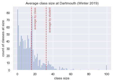
This isn’t just a quirk of my toy example. If we look at Dartmouth’s class enrollment for winter 2019, we can see that the average class size and the observed class size for a student are substantially different.

import pandas

courses = pandas.read_html(
    "../assets/dartmouth-winter-2019-enrollment.html",
    "Instructor")[2]
class_sizes = courses.Enrl

import matplotlib.pyplot as plt
import seaborn as sns
sns.set()

%matplotlib inline

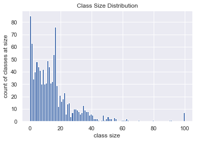
clipped_class_sizes = class_sizes.clip(0, 100)
plt.hist(clipped_class_sizes,
         bins=clipped_class_sizes.max())
plt.title("Class Size Distribution")
plt.xlabel("class size")
plt.ylabel("count of classes at size");

To calculate the average class size as observed by a student, we can draw random classes from the list of classes weighted by their enrollment, kind of like picking a course-load by randomly selecting seats in distinct classes.

import numpy

# I generate each student's classes
# independently in a loop so that I
# can use replace=False and prevent
# anyone from attending the same class
# multiple times

SIMULATED_STUDENTS = 1000

average_observed_class_size = numpy.vstack([
    numpy.random.choice(
        class_sizes,
        p=class_sizes / class_sizes.sum(),
        size=3,  # typical courseload
        replace=False)  # can't attend same class twice
    for _ in range(SIMULATED_STUDENTS)
]).mean(axis=1)

plt.hist(average_observed_class_size, bins=100)
plt.title("Estimated observed class size")
plt.xlabel("class size")
plt.ylabel("students who observed");

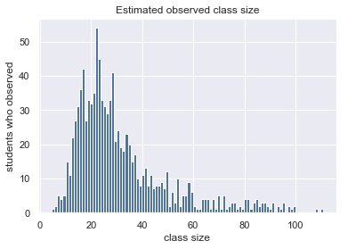
The simulation above assigns each student a list of class sizes like (30, 14, 61) that they observed. In a full simulation, with each class filling up, there would be 30 data-points for a class with size 30, 5 for a class with size 5, … which makes the calculation much simpler. Instead of averaging sum(class sizes) / 3 over all students, we can combine the numerators to get

average_by_student = (class_sizes ** 2).sum() \
                     / class_sizes.sum()
average_by_student

32.44172932330827

If we take the average by class instead, it appears much better

average_by_class = class_sizes.replace(0, numpy.nan).mean()
average_by_class

15.896414342629482

I couldn’t find an average class size figure, but I did find a breakdown of classes by size which indicates:

• 64.5% of classes are < 20 students
• 28.6% of classes are 20-49 students
• 6.9% of classes are >= 50 students

bucketed = pandas.cut(class_sizes,
                      [-numpy.inf, 19, 49, numpy.inf])

class_buckets = (
  bucketed.value_counts() / len(bucketed)
).to_frame(name="based on winter 2019")
class_buckets.index.name = "class size bucket"
class_buckets['official count'] = [0.645, 0.286, 0.069]
class_buckets.style.format("{:.0%}")

	based on winter 2019	official count
class size bucket
(-inf, 19.0]	77%	64%
(19.0, 49.0]	20%	29%
(49.0, inf]	3%	7%

clipped_class_sizes = class_sizes.clip(0, 100)

plt.hist(clipped_class_sizes,
         clipped_class_sizes.max(),
         alpha=0.4)

top = clipped_class_sizes.value_counts().max()

plt.axvline(average_by_student, color="r", linestyle="--")
plt.text(average_by_student + 3,
         top,
         "average by student",
         rotation=90,
         color="r");

plt.axvline(average_by_class, color="r", linestyle="--")
plt.text(average_by_class + 3,
         top,
         "average by class",
         rotation=90,
         color="r");

plt.title("Average class size at Dartmouth (Winter 2019)")
plt.xlabel("class size")
plt.ylabel("count of classes at size");